Background
I used to hear many people talk about that fast fourier transform (FFT) is one of the most beautiful algorithms in the engineering world, but I never dove deep into that.
Then a few days ago I stumble upon this wonderful Youtube video about FFT created by @Reducible. So I took some note of my learning from the that video. I figured out this note is probably qualified for public consumption so I decided to publicize it.
If you haven’t watched the video yet, I highly recommend you to watch it:
- The Fast Fourier Transform (FFT): Most Ingenious Algorithm Ever? - YouTube
- FFT Example: Unraveling the Recursion - YouTube
Let’s begin the journey!
Polynomial multiplication problem
How do we multiply two polynomials? A method we all learned from high school is to use distribution law to expand the terms, and then combine the terms with the same exponent. Here’s an example:
\[\begin{equation} \begin{split} (5x^2+4)(2x^2+x+1) & = 5x^2(2x^2+x+1) + 4(2x^2+x+1) \\ & = (10x^4+5x^3+5x^2) + (8x^2+4x+4) \\ & = 10x^4+5x^3+13x^2+4x+4 \\ \end{split} \end{equation} \]Polynomial representation
If we want to implement the multiplication in a program, we first need to find a way to represent the polynomial.
For polynomial of degree \(d\), there are two unique ways we can use:
- use a list \(d+1\) of coefficients of the powers: \([p_0, p_1, ..., p_d]\) (coefficient representation)
- use a set of \(d+1\) distinct points: \({(x_0, P(x_0)), (x_1, P(x_1)), ..., (x_d,P(x_d))}\) (value representation)
The value representation works because a polynomial of degree \(N\) can be determined by \(N+1\) distinct interpolation points. For example, two points determine a line, three points determine a parabola.
The coefficient representation is what we demonstrated in Polynomial multiplication problem. It’s straightforward and we already know it. However, it’s not performant enough for polynomial multiplication. The time complexity is \(O(N^2)\) where \(N\) is the degree of the polynomial, because we need to multiply all possible pairs of terms.
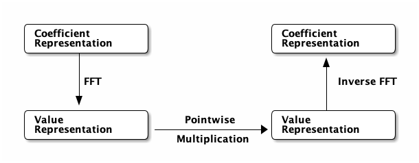
The value representation, on the other hand, is much faster for multiplying polynomial. To multiply two polynomials, if we assume the \(\mathbf{x}\) values are consistent in the two representations, we can just pointwise multiply the \(P(\mathbf{x})\) values. So this algorithm has a time complexity of \(O(N)\).
Flowchart for polynomial multiplication
Now we can draw a diagram on how to perform fast multiplication for polynomials. The step involved in converting coefficient representation into value reprentation is where fast fourier transform (FFT) kicks in.
Coefficient representation conversion
The most naive method to convert coefficient representation is just to plug in some arbitrary values to the polynomial.
However, this will result in us going back to the original complexity because we need to calculate for each term in the polynomial and for each \(x\) value. This will get us back to \(O(N^2)\) time complexity with \(N\) being the degree of the polynomial. Not good.
This is where Fast Fourier Transform algorithm shines. The FFT algorithm is able do the same conversion in just \(O(N \log N)\) time!
We will learn about the tricks FFT based on and see if we can derive FFT ourselves.
Polynomial evaluation
First, let’s see how we can improve the naive algorithm. Suppose we have a polynomial term of even power, \(5x^2\) for example, then we can carefully pick the \(\mathbf{x}\) points to be symmetrical about the \(y\) axis. If we do so, we only need to perform half the computation since once we know \(P(x)\), we automatically know \(P(-x) = P(x)\). Similarly, for individual odd degree terms, we have \(P(x)=-P(-x)\).
With this trick, we can cut the number of computations needed by half. For each individual point \(x_i\), to compute \(P(x_i)\), we can split the calculation into \(P_e(x_i^2)\) and \(x_i P_o(x_i^2)\) which represent the even and odd degree terms, respectively.
For example, \(P(x) = 5x^5 + 6x^4 + 7x^3 + 8x^2 + 9x + 10\) evaluated at \(x_i\) can be written as \(P_e(x_i^2) + x P_o(x_i^2)\), where \(P_e(x^2) = 6x^4 + 8x^2 + 10\) and \(P_o(x^2) = 5x^5 + 7x^3 + 9x\).
Then we have:
\[\begin{equation} \begin{cases} P( x_i) &= P_e(x_i^2) + x_i P_o(x_i^2) \\ P(-x_i) &= P_e(x_i^2) - x_i P_o(x_i^2) \end{cases} \end{equation} \]In which \(P_e(x_i^2)\) and \(P_o(x_i^2)\) can be calculated only once and used twice.
From here we can go with the recursive step. \(P_e(x)\) and \(P_o(x)\) each is a polynomial of degree \(d/2\), which only have half of the terms. We can further apply the algorithm to it with half the size until we reach the base case where \(d=0\). In such case we just have \(1\) term - the constant term, so we can just return it as the evaluation result.
Except there is a blocker in the recursion step. The “divide” step works based on the assumption that we can always choose two set of points \(\mathbf{x_i}\) and \(-\mathbf{x_i}\). This will not be the case except for the first iteration. In the second iteration we will have \(x_i^2\) and \((-x_i)^2\) which are normally both positive, so we can no longer further split the polynomial - well, unless we introduce complex number into the play.
Constraints for the sample points
Let’s list out the requirements we need for the \(N\) sampling points for degree \(N-1\) polynomial. From now on, for simplicity purpose, we will only talk about polynomial with degree \(2^k-1\) where \(k\in\mathbb{Z}^{*}\).
In the first iteration, we have \(N\) points, half of them need to be negation of the other half. Let’s note down the conditions.
\[\label{cond1} x_{\frac{N}{2}+i} = -x_i\quad\text{for } i \in 0,\ldots,\frac{N}{2}\]
Note that we only need to compute half of the point set.
Then in the next interation, we will be passing \(x_k^2\) to the \(P_e\) and \(P_o\), where \(k\) takes values of \(0,..,N/4\).
\[\label{cond2} x_{\frac{N}{4}+i}^2 = -x_i^2\quad\text{for }i \in 0,\ldots,\frac{N}{4}\]
Starting from equations and we can inductively deduce all the restrictions on all \(x\) values.
The base case for polynomial of degree \(N-1\) is \(x_0^{N}\). We can assign it to \(x_0^N = 1\). This value specifies \(x_0^{\frac{N}{2}}\) and \(x_1^{\frac{N}{2}}\) to be the two roots of \(x_0^N\) that are negation of each other. In the next iteration, each of these two values in turn specifies four more values, \(x_i^{\frac{N}{4}}\) for \(i\in \{0,1,2,3\}\) and so on. Until we hit the case \(\frac{N}{2^k} = 1\), then we get all the plain \(x_i^{\frac{N}{2^k}}=x_i\) values.
Let’s look at the second interation, where we acquired the constraint that \(x_0^{\frac{N}{2}}\) and \(x_1^{\frac{N}{2}}\) are roots of \(x_0^N=1\), so one must be \(1\) and other be \(-1\). But in reality they can be of any order. Same choice must be made to all future iterations.
The trick is to take \(x_i\) to be the \(i\) th element of the “\(N\) th root of unity”.
\[\begin{equation} x_i=e^{2\pi j\frac{i}{N}} \end{equation} \]Where \(j=\sqrt{-1}\). We can verify that these points satisfy the constraints we wanted: \(x_0^N=e^{0}=1\); then \(x_0^{N/2} = e^{0} = 1\) and \(x_1^{N/2}=e^{\pi j} = -1\) are the roots of \(x_0^N\); and so on.
Symmetrical properties of sample points
If we plot the points for \(e^{2\pi j \frac{i}{N}}\) for all \(i\) on the complex plane, we can find that they reside on a circle with equal distance apart. Here’s a graph for \(N=8\).
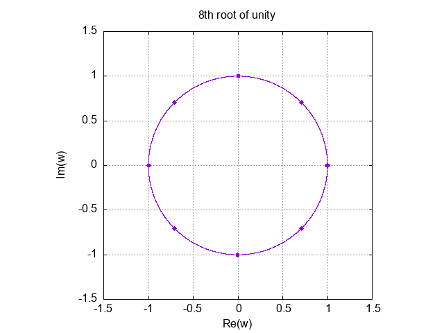
The \(x\) points are arranged in an counter-clockwise order, starting from \(x_0=1\).
We can see that these points are symmetrical about the origin - that is to say, every point \(x_i\) has a counterpart \(x_{N/2+i}=-x_i\), which is the reflection of \(x_i\) about the origin. This property is exactly what we wanted.
In the following iterations, we would square the half of all the \(x_i\) values. Squaring a unit complex number \(z\) is the same as doubling angle of the number couter-clockwise. So in the next iterations, we essentially continue to fill the circle with half of the points, resulting a new circle where points are twice the old distance apart. In the last iteration, the result will be just a single point \(x_0^N = 1\).
Constructing the algorithm
We now learned how to pick sample points, now let’s formalize the algorithm.
The FFT algorithm should take two arguments, a list of coefficients representing the polynomial, and a list of sampling points. The output is a list of \(P(x_i)\) values corresponding to each point \(x_i\). \(N\) is represented by the length of the coefficient list (or the number of points, which is the same anyway).
The simplest case is when \(N=1\), where we have to calculate \(\operatorname{FFT}(P=[c_0], X=[1])\), which is the same as evaluating \(P(x)=c_0\) at \(x=1\). The result is trivial - we just return \(Y=[c_0]\).
Next simplest case is when \(N=2\), where we have \(\operatorname{FFT}(P=[c_0, c_1], X=[1, -1])\). This polynomial is easy to calcualte on its own. Although the recursive algorithm applies at this case, it’s not very representative for demonstration purpose, so we will skip this iteration and assume it works normally.
The next one is \(N=3\), where we have \(\operatorname{FFT}(P=[c_0, c_1, c_2, c_3], X=[1, j, -1, -j])\), that is, to evaluate \(c_0 + c_1 x^1 + c_2 x^2 + c_3 x^3\) at the given \(x_i\) points.
We first split \(P(x)\) into even and odd components: \(P_e(x^2)+xP_o(x^2) = (c_0+c_2 x^2) + x(c_1+c_3 x^2)\). This gave us two smaller polynomials for the recursion step \(P_e=[c_0, c_2]\) and \(P_o = [c_1, c_3]\).
Now let’s see what \(x_i\) values we need to provide for the recursion step. The whole point of the algorithm is to save half of the calculation by exploiting the even/odd polynomials. So we only need to calculate for these polynomials on \(X=[1, j]\). Note that their arguments are not \(x_i\) but \(x_i^2\). So we need to pass \(X=[1, j^2=-1]\) to them. The same parameter applies to both the even and odd polynomials. In turn, we are left with evaluating two expressions \(Y_e = \operatorname{FFT}(P=[c_0, c_2], X=[1, -1])\) and \(Y_o=\operatorname{FFT}(P=[c_1, c_3], X=[1, -1])\). This reduces our problem of size \(N=4\) to two \(N=2\) cases.
Now comes the final part - after we computed the \(Y_e\) and \(Y_o\), we need to compose them in a way that calculates the final \(Y\) values. Given that \(x_{N/2+i}=-x_i\) for \(i \in 0,..,\frac{N}{2}\), and the nature of even/odd polynomials, we know that \(P_e(x_{N/2+i})=P_e(x_i)\) and \(P_o(x_{N/2+i}) = -P_o(x_i)\). Also we know \(P=P_e + x P_o\). This gave us the way to compose the \(Y_e\) and \(Y_o\). \(y_i = y_e+ x_i y_i\) and \(y_{N/2+i} = y_e - x_i y_i\) for \(i \in 0,..,\frac{N}{2}\).
Now we can observe another invariant. For all recursion steps, the \(X\) values for that step are fixed. In other words, the values of \(X\) only depend on the degree \(N\), which can be deduced from length of the coefficient list. For \(N=1\), we always have \(X=[1]\); for \(N=2\), we always have \(X=[1,-1]\); for \(N=4\), we always have \(X=[1,j,-1,-j]\). This result comes from our previous reasoning from last section about squaring roots of unity. As a result, we no longer have to explicitly specify this argument to FFT procedure.
Implementing in code
To implement the algorithm in code, we basically just copy the steps described above. Note that we represent \(x_i=e^{2 \pi j \frac{i}{N}}\) with \(w^i\) where \(w=e^{2 \frac{\pi j}{N}}\).
import math
import cmath

def fft(p):
  n = len(p)
  if n == 1:
    return p
  w = cmath.exp(2*math.pi*1j/n)
  y_e = fft(p[0::2])
  y_o = fft(p[1::2])
  y = [None] * n
  for i in range(n//2):
    y[i]      = y_e[i] + y_o[i] * w**i
    y[i+n//2] = y_e[i] - y_o[i] * w**i
  return y
Let’s verify if the result is correct.
def p(x):
  return 1 + 2*x + 3*x**2 + 4*x**3

print(fft([1,2,3,4]))
print([p(1), p(1j), p(-1), p(-1j)])
[(10+0j), (-2-2j), (-2+0j), (-1.9999999999999998+2j)]
[10, (-2-2j), -2, (-2+2j)]
Ignoring the round-off error, we can see the two results are the same.
FFT operation as a matrix
The naive method of evaluating the value of a polynomial of degree \(N-1\) at \(N\) sampling points is to calculating \(N\) values, which are \(P(x_i)\) where \(i = 0, 1, \ldots, N-1\). Then, to calculate \(P(x_i)\), we need to sum up the the value of each terms
\[\begin{equation} P(x_i) = \sum_{k=0}^{N-1} x_i^kc_k \end{equation} \]where \(c_k\) is the k-th coefficient of the polynomial. This means we can construct an \(N\) by \(N\) matrix with each element to be \(W_{i,k} = x_i^k\).
\[\begin{equation} W = \begin{pmatrix} 1 & x_0 & x_0^2 & \cdots & x_0^m \\ 1 & x_1 & x_1^2 & \cdots & x_1^m \\ 1 & x_2 & x_2^2 & \cdots & x_2^m \\ \vdots & \vdots & \vdots & \ddots & \vdots \\ 1 & x_m & x_m^2 & \cdots & x_m^m \\ \end{pmatrix} \end{equation} \]where \(m = N-1\). If we plug in our chosen sampling points \(x_i = w^i = e^{\frac{2\pi j}{n}}\) we get this matrix:
\[\begin{equation} W = \begin{pmatrix} 1 & 1 & 1 & \cdots & 1 \\ 1 & w & w^2 & \cdots & w^m \\ 1 & w^2 & w^4 & \cdots & w^{2m} \\ 1 & w^3 & w^6 & \cdots & w^{3m} \\ \vdots & \vdots & \vdots & \ddots & \vdots \\ 1 & w^m & w^{2m} & \cdots & w^{m^2} \\ \end{pmatrix} \end{equation} \]Given a vector of coefficient \(P=[c_0, c_1, \ldots, c_m]\), the result of \(Y = WP\) is just the sampled values we wanted.
In fact, this matrix is called the discrete fourier transform matrix (DFT matrix) for this exact reason. The FFT algorithm above is just an more efficient way to perform the matrix multiplication with this matrix.
Correspondingly, the technique to calculate the inverse fourier transform is to find the inverse matrix. And interestingly, the inverse DFT matrix looks very similar to the DFT matrix!
\[\begin{equation} W^{-1} = \frac{1}{N}\begin{pmatrix} 1 & 1 & 1 & \cdots & 1 \\ 1 & w^{-1} & w^{-2} & \cdots & w^{-m} \\ 1 & w^{-2} & w^{-4} & \cdots & w^{-2m} \\ 1 & w^{-3} & w^{-6} & \cdots & w^{-3m} \\ \vdots & \vdots & \vdots & \ddots & \vdots \\ 1 & w^{-m} & w^{-2m} & \cdots & w^{-m^2} \\ \end{pmatrix} \end{equation} \]The fact that the inverse DFT matrix is similar to the DFT matrix gives us a way to compute inverse fast fourier transform. This means to convert our FFT algorithm to Inverse FFT algorithm, we only need the following two changes,
- replace all occurences \(w\) with \(w^{-1}\);
- finally, multiply with \(\frac{1}{N}\).
Implementation of Inverse FFT algorithm
And - here we have it.
def _ifft(p):
  n = len(p)
  if n == 1:
    return p
  w = cmath.exp(-2*math.pi*1j/n)
  y_e = _ifft(p[0::2])
  y_o = _ifft(p[1::2])
  y = [None] * n
  for i in range(n//2):
    y[i]      = y_e[i] + y_o[i] * w**i
    y[i+n//2] = y_e[i] - y_o[i] * w**i
  return y

def ifft(p):
  n = len(p)
  return [x/n for x in _ifft(p)]
Now let’s try out if it’s indeed the inverse of fft function.
print(ifft(fft([1,2,3,4])))
print(fft(ifft([1j,2j+1])))
[(1+0j), (2-5.721188726109833e-18j), (3+0j), (4+5.721188726109833e-18j)]
[1j, (1+2j)]
Ihe inverse does seem to work ignoring the round-off errors.
I tried to understand the IFFT algorithm in a similar way as we exploit the symmetry of even and odd polynomials, but I can’t find a way to make sense of it. The algorithm itself still works like magic - I can’t explain it with a deeper understanding. I am sorry if you’re expecting that.
Polynomial multiplication
Now we have all the components in the flowchart, we can finally implement the algorithm to perform fast polynomial multiplication.
def pad_radix2(xs, n):
    b = n.bit_length() - 1
    if n & (n-1): # not a power of 2
        b += 1
        n = 2 ** b
    return xs + [0] * (n - len(xs))

def poly_mult(p1, p2):
    max_n = max(len(p1), len(p2)) * 2
    y1, y2 = fft(pad_radix2(p1, max_n)), fft(pad_radix2(p2, max_n))
    y3 = [a * b for a, b in zip(y1, y2)]
    return ifft(y3)

# calculate (2x+1)(4x+3)
print(poly_mult([1,2], [3,4]))
[(3+8.881784197001252e-16j), (10-3.599721149882556e-16j), (8-8.881784197001252e-16j), 3.599721149882556e-16j]
3,10,8 - we just calculated that \((2x+1)(4x+3)=8x^2 + 10x + 3\). The algorithm worked!
Summary
In this article we studied how to make use of FFT algorithm to compute polynomial multiplication in \(O(N \log N)\) time. We mainly studied how the ingenious tricks work together to make FFT algorithm concise and elegant, and finally implemented the multiplication algorithm in code.
References
This article is mainly my personal note on Reducible’s fantastic video The Fast Fourier Transform (FFT): Most Ingenious Algorithm Ever? on Youtube. Huge thanks to Reducible for the presentation.
Some other sources that are helpful for my understanding:
- Source code of
fftfunction in sympy. I learned how to quickly pad up a list to radix-2 length. - jakevdp’s post “Understanding the FFT Algorithm”. I learned the trick
numpyuses to make it much faster than my implementation. - This math stackexchange answer. It resolved my confusion on the discrepancy of the formula on Wikipedia and the formula used in the video.